PyTorch 01 - Tensors

PyTorch Introduction

PyTorch is an open-source machine learning library developed by Facebook’s AI Research lab.

It is widely used for deep learning tasks, particularly in the field of natural language processing (NLP) and computer vision.

Started at Facebook AI Research (FAIR), now Fundamntal AI Research, to build a consolidated tool for deep learning tasks.

2015 there was Theano (Montreal) Caffe (Berkeley) and Lua Torch (FAIR).
2015 December, Google released TensorFlow
~2016 Released Caffe2 for targeting mobile and edge devices (Facebook Production)
2015-2016 FAIR refactored Torch to separate computation backend from frontend and create a new frontend in Pythyon
- the core library is still called torch
Sep 2016 PyTorch v0.1.1 released (torch.nn and torch.autograd modules)
Dec 2018 PyTorch v1.0 released (Replace Caffe2 for FB production)
Mar 15 2023 PyTorch v2.0 released (dynamic shapes, distributed training, Transformers support, etc.)
(Latest Release)Aug 2024 PyTorch 2.4.1

Key Features of PyTorch

Dynamic Computation Graph: PyTorch’s dynamic computation graph allows for more intuitive and flexible model building. This means that the graph is constructed at runtime, allowing for more dynamic and interactive model development.
GPU and TPU Acceleration: PyTorch can leverage GPUs and TPUs for accelerated training, making it faster than many other deep learning frameworks.
Autograd: PyTorch’s autograd module provides automatic differentiation, which allows for easy computation of gradients and updates to model parameters during training.
High-Level API: PyTorch has a high-level API that allows for easy model building and training. It also has a low-level API that provides more control over the model building process.

PyTorch vs TensorFlow

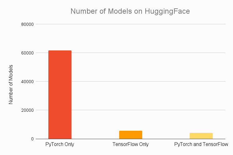
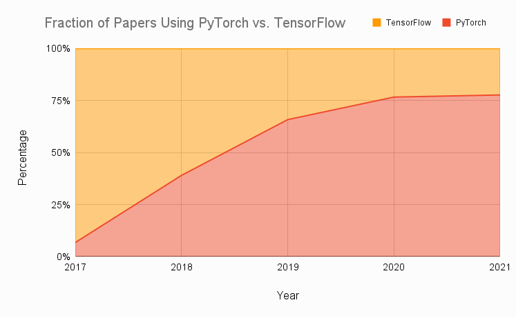
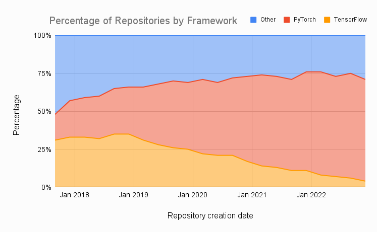
From https://www.assemblyai.com/blog/pytorch-vs-tensorflow-in-2023/.

Key Differences

PyTorch

Dynamic Computation Graph
Autograd
High-Level API
Arguably more “pythonic”

TensorFlow

Static Computation Graph
Eager Execution
Low-Level API (high-level API is Keras)

Tutorial

We’ll borrow heavily from https://pytorch.org/tutorials/ and other sources that we’ll cite.

Tensors

Fundamentally, PyTorch tensor is a data structure for storing matrices and multi-dimensional arrays.

Similar to NumPy’s ndarrays.

But it does much more.

Manages translation to accelerator data formats and hardware memory
Stores information needed for automatic gradient (autograd) calculation for parameter updates
etc…

import torch
import numpy as np

Tensor Creation

We have to get data into PyTorch tensors before we can operate on them.

There are multiple ways to do that.

Create directly from a Python list such as this one:

data = [[1, 2], [2, 3]]
print(f"data: {data}")
print(f"type(data): {type(data)}")

data: [[1, 2], [2, 3]]
type(data): <class 'list'>

Create the tensor and explore some of its attributes.

x_data = torch.tensor(data)
print(f"x_data: {x_data}")
print(f"type(x_data): {type(x_data)}")
print(f"x_data.dtype: {x_data.dtype}")
print(f"x_data.shape: {x_data.shape}")
print(f"x_data.device: {x_data.device}")
print(f"x_data.requires_grad: {x_data.requires_grad}")
print(f"x_data.is_leaf: {x_data.is_leaf}")

x_data: tensor([[1, 2],
        [2, 3]])
type(x_data): <class 'torch.Tensor'>
x_data.dtype: torch.int64
x_data.shape: torch.Size([2, 2])
x_data.device: cpu
x_data.requires_grad: False
x_data.is_leaf: True

As mentioned, some of the interesting attributes are:

x_data.device: The device where the tensor is stored.
x_data.requires_grad: Whether the tensor requires gradient computation.
x_data.is_leaf: Whether the tensor is a leaf node in the computation graph.

We’ll get more into these later.

If we use decimal numbers, then a floating point number type is chosen.

y_data = torch.tensor([[0.1, 1.2], [2.2, 3.1]])
print(f"y_data: {y_data}")
print(f"y_data.dtype: {y_data.dtype}")
print(f"y_data.device: {y_data.device}")

y_data: tensor([[0.1000, 1.2000],
        [2.2000, 3.1000]])
y_data.dtype: torch.float32
y_data.device: cpu

From a NumPy array

np_array = np.array(data)
x_np = torch.from_numpy(np_array)

As the same shape of another tensor

x_ones = torch.ones_like(x_data) # retains the properties of x_data
print(f"Ones Tensor: \n {x_ones} \n")

x_rand = torch.rand_like(x_data, dtype=torch.float) # overrides the datatype of x_data
print(f"Random Tensor: \n {x_rand} \n")

Ones Tensor: 
 tensor([[1, 1],
        [1, 1]]) 

Random Tensor: 
 tensor([[0.1395, 0.9440],
        [0.8645, 0.1542]])

With random or constant values

shape = (2,3)
rand_tensor = torch.rand(shape)
ones_tensor = torch.ones(shape)
zeros_tensor = torch.zeros(shape)

print(f"Random Tensor: \n {rand_tensor} \n")
print(f"Ones Tensor: \n {ones_tensor} \n")
print(f"Zeros Tensor: \n {zeros_tensor}")

Random Tensor: 
 tensor([[0.6207, 0.7855, 0.7596],
        [0.1035, 0.8634, 0.9637]]) 

Ones Tensor: 
 tensor([[1., 1., 1.],
        [1., 1., 1.]]) 

Zeros Tensor: 
 tensor([[0., 0., 0.],
        [0., 0., 0.]])

Tip

There are many more creation functions listed in Creation Ops for things like sparse tensors, other random number generators, etc.

Operations on Tensors

Let’s look at some interesting operations we can perform on tensors.

Standard numpy-like indexing and slicing

Python itself has some flexible indexing and slicing support. See this tutorial for a nice overview.

PyTorch follows the NumPy indexing and slicing conventions.

# Define a 4x4 tensor
tensor = torch.tensor([[1, 2, 3, 4], [5, 6, 7, 8], [9, 10, 11, 12], [13, 14, 15, 16]], dtype=torch.float32)
#tensor = torch.ones(4, 4)
print(f"tensor.dtype: {tensor.dtype}")

# Matrices are stored in row-major order, and like NumPy, it is a list of lists.
print(f"First row: {tensor[0]}")
print(f"Second row: {tensor[1]}")

# Like python we use `:` to index and slice
print(f"First column: {tensor[:, 0]}")
print(f"Second column: {tensor[:, 1]}")

# Slicing with `...` is a shortcut for "all remaining dimensions"
print(f"Last column: {tensor[..., -1]}")
print(f"Last column: {tensor[:, -1]}")

# There is also broadcasting support
tensor[:,1] = 0
print(tensor)

tensor.dtype: torch.float32
First row: tensor([1., 2., 3., 4.])
Second row: tensor([5., 6., 7., 8.])
First column: tensor([ 1.,  5.,  9., 13.])
Second column: tensor([ 2.,  6., 10., 14.])
Last column: tensor([ 4.,  8., 12., 16.])
Last column: tensor([ 4.,  8., 12., 16.])
tensor([[ 1.,  0.,  3.,  4.],
        [ 5.,  0.,  7.,  8.],
        [ 9.,  0., 11., 12.],
        [13.,  0., 15., 16.]])

Joining tensors

You can use torch.cat to concatenate a sequence of tensors along a given dimension. See also torch.stack, another tensor joining operator that is subtly different from torch.cat.

t1 = torch.cat([tensor, tensor, tensor], dim=1)
print(t1)

tensor([[ 1.,  0.,  3.,  4.,  1.,  0.,  3.,  4.,  1.,  0.,  3.,  4.],
        [ 5.,  0.,  7.,  8.,  5.,  0.,  7.,  8.,  5.,  0.,  7.,  8.],
        [ 9.,  0., 11., 12.,  9.,  0., 11., 12.,  9.,  0., 11., 12.],
        [13.,  0., 15., 16., 13.,  0., 15., 16., 13.,  0., 15., 16.]])

t2 = torch.cat([tensor, tensor, tensor], dim=0)
print(t2)

tensor([[ 1.,  0.,  3.,  4.],
        [ 5.,  0.,  7.,  8.],
        [ 9.,  0., 11., 12.],
        [13.,  0., 15., 16.],
        [ 1.,  0.,  3.,  4.],
        [ 5.,  0.,  7.,  8.],
        [ 9.,  0., 11., 12.],
        [13.,  0., 15., 16.],
        [ 1.,  0.,  3.,  4.],
        [ 5.,  0.,  7.,  8.],
        [ 9.,  0., 11., 12.],
        [13.,  0., 15., 16.]])

Matrix Multiplication

Matrix multiplication is a fundamental operation in deep learning and PyTorch provides a number of ways to perform it.

Equivalent matrix multiplication operations

We’ll use the following helper function to format the tensors as LaTeX matrices.

Code

import torch
from IPython.display import display, Math

def tensor_to_latex(tensor):
    """Convert a PyTorch tensor to a LaTeX bmatrix string."""
    if tensor.dim() == 1:
        # Convert 1D tensor to a 2D column vector for display
        tensor = tensor.unsqueeze(1)
    
    latex_str = "\\begin{bmatrix}\n"
    for row in tensor:
        latex_str += " & ".join([f"{val.item():.2f}" for val in row]) + " \\\\\n"
    latex_str += "\\end{bmatrix}"
    return latex_str

# Define matrix A and vector x
A = torch.tensor([[1.0, 2.0], [3.0, 4.0]])
x = torch.tensor([5.0, 6.0])

# Compute the product A * x
Ax = torch.matmul(A, x)

# Convert tensors to LaTeX
latex_A = tensor_to_latex(A)
latex_x = tensor_to_latex(x)
latex_Ax = tensor_to_latex(Ax)

# Display the equation A x = Ax on one line
display(Math(f"A \\times x = {latex_A} \\times {latex_x} = {latex_Ax}"))

\(\displaystyle A \times x = \begin{bmatrix} 1.00 & 2.00 \\ 3.00 & 4.00 \\ \end{bmatrix} \times \begin{bmatrix} 5.00 \\ 6.00 \\ \end{bmatrix} = \begin{bmatrix} 17.00 \\ 39.00 \\ \end{bmatrix}\)

We’ll use the tensor from before.

Code

latex_tensor = tensor_to_latex(tensor)
display(Math(f"\\mathrm{{tensor}} = {latex_tensor}"))

\(\displaystyle \mathrm{tensor} = \begin{bmatrix} 1.00 & 0.00 & 3.00 & 4.00 \\ 5.00 & 0.00 & 7.00 & 8.00 \\ 9.00 & 0.00 & 11.00 & 12.00 \\ 13.00 & 0.00 & 15.00 & 16.00 \\ \end{bmatrix}\)

There are three different ways shown below that produce the same result.

Method 1: Use the `@` matrix multiplication operator

# ``tensor.T`` returns the transpose of a tensor
y1 = tensor @ tensor.T
# print(f"y1: {y1}")

latex_tensorT = tensor_to_latex(tensor.T)
latex_y1 = tensor_to_latex(y1)
display(Math(f"y1 = \\mathrm{{tensor}} \\times \\mathrm{{tensor.T}} = {latex_tensor} \\times {latex_tensorT} = {latex_y1}"))

\(\displaystyle y1 = \mathrm{tensor} \times \mathrm{tensor.T} = \begin{bmatrix} 1.00 & 0.00 & 3.00 & 4.00 \\ 5.00 & 0.00 & 7.00 & 8.00 \\ 9.00 & 0.00 & 11.00 & 12.00 \\ 13.00 & 0.00 & 15.00 & 16.00 \\ \end{bmatrix} \times \begin{bmatrix} 1.00 & 5.00 & 9.00 & 13.00 \\ 0.00 & 0.00 & 0.00 & 0.00 \\ 3.00 & 7.00 & 11.00 & 15.00 \\ 4.00 & 8.00 & 12.00 & 16.00 \\ \end{bmatrix} = \begin{bmatrix} 26.00 & 58.00 & 90.00 & 122.00 \\ 58.00 & 138.00 & 218.00 & 298.00 \\ 90.00 & 218.00 & 346.00 & 474.00 \\ 122.00 & 298.00 & 474.00 & 650.00 \\ \end{bmatrix}\)

Method 2: call `.matmul` method on the tensor

y2 = tensor.matmul(tensor.T)
# print(f"y2: {y2}")

latex_y2 = tensor_to_latex(y2)
display(Math(f"y2 = \\mathrm{{tensor}} \\times \\mathrm{{tensor.T}} = {latex_tensor} \\times {latex_tensorT} = {latex_y2}"))

\(\displaystyle y2 = \mathrm{tensor} \times \mathrm{tensor.T} = \begin{bmatrix} 1.00 & 0.00 & 3.00 & 4.00 \\ 5.00 & 0.00 & 7.00 & 8.00 \\ 9.00 & 0.00 & 11.00 & 12.00 \\ 13.00 & 0.00 & 15.00 & 16.00 \\ \end{bmatrix} \times \begin{bmatrix} 1.00 & 5.00 & 9.00 & 13.00 \\ 0.00 & 0.00 & 0.00 & 0.00 \\ 3.00 & 7.00 & 11.00 & 15.00 \\ 4.00 & 8.00 & 12.00 & 16.00 \\ \end{bmatrix} = \begin{bmatrix} 26.00 & 58.00 & 90.00 & 122.00 \\ 58.00 & 138.00 & 218.00 & 298.00 \\ 90.00 & 218.00 & 346.00 & 474.00 \\ 122.00 & 298.00 & 474.00 & 650.00 \\ \end{bmatrix}\)

Method 3: Call the `torch.matmul` function with the two input operands and the output tensor.

# This creates a new tensor with the same shape and type as y1, filled with random numbers from a uniform distribution over [0, 1)
y3 = torch.rand_like(y1)
#print(f"y3: {y3}")

torch.matmul(tensor, tensor.T, out=y3)
# print(f"y3: {y3}")

latex_y3 = tensor_to_latex(y3)
display(Math(f"y3 = \\mathrm{{torch.matmul(tensor, tensor.T)}} = {latex_tensor} \\times {latex_tensorT} = {latex_y3}"))

\(\displaystyle y3 = \mathrm{torch.matmul(tensor, tensor.T)} = \begin{bmatrix} 1.00 & 0.00 & 3.00 & 4.00 \\ 5.00 & 0.00 & 7.00 & 8.00 \\ 9.00 & 0.00 & 11.00 & 12.00 \\ 13.00 & 0.00 & 15.00 & 16.00 \\ \end{bmatrix} \times \begin{bmatrix} 1.00 & 5.00 & 9.00 & 13.00 \\ 0.00 & 0.00 & 0.00 & 0.00 \\ 3.00 & 7.00 & 11.00 & 15.00 \\ 4.00 & 8.00 & 12.00 & 16.00 \\ \end{bmatrix} = \begin{bmatrix} 26.00 & 58.00 & 90.00 & 122.00 \\ 58.00 & 138.00 & 218.00 & 298.00 \\ 90.00 & 218.00 & 346.00 & 474.00 \\ 122.00 & 298.00 & 474.00 & 650.00 \\ \end{bmatrix}\)

There is additional behavior depending on the dimensionality of the tensors.

Vector Dot Product

If both tensors are 1-D, then the vector dot product is performed.

torch.manual_seed(0)

# vector x vector
tensor1 = torch.randint(low=0, high=10, size=(3,))
tensor2 = torch.randint(low=0, high=10, size=(3,))
# print(f"tensor1: {tensor1} and tensor2: {tensor2}")

latex_tensor1 = tensor_to_latex(tensor1)
latex_tensor2 = tensor_to_latex(tensor2)

display(Math(f"\\mathrm{{tensor1}} = {latex_tensor1}, \\mathrm{{tensor2}} = {latex_tensor2}"))


tensor3 = torch.matmul(tensor1, tensor2)
print(f"tensor3 = tensor1 @ tensor2: {tensor3}")
print(f"tensor3.size(): {tensor3.size()}")

\(\displaystyle \mathrm{tensor1} = \begin{bmatrix} 4.00 \\ 9.00 \\ 3.00 \\ \end{bmatrix}, \mathrm{tensor2} = \begin{bmatrix} 0.00 \\ 3.00 \\ 9.00 \\ \end{bmatrix}\)

tensor3 = tensor1 @ tensor2: 54
tensor3.size(): torch.Size([])

So with 1-D tensors, torch.matmul and torch.dot are equivalent.

tensor3 = torch.dot(tensor1, tensor2)
print(f"tensor3 = torch.dot(tensor1, tensor2): {tensor3}")
print(f"tensor3.size(): {tensor3.size()}")

tensor3 = torch.dot(tensor1, tensor2): 54
tensor3.size(): torch.Size([])

Matrix-Vector Multiplication

Now let’s look at the case where one operand is 1D and the other is 2D.

If the first argument is 2-dimensional and the second argument is 1-dimensional, the matrix-vector product is returned.

tensor1 = torch.tensor([[1, 2], [3, 4]])
print(f"Operand 1 --tensor1.size(): {tensor1.size()}")
# print(f"Operand 1 -- tensor1: {tensor1}")
latex_tensor1 = tensor_to_latex(tensor1)

tensor2 = torch.tensor([1, 2])
print(f"Operand 2 --tensor2.size(): {tensor2.size()}")
#print(f"Operand 2 --tensor2: {tensor2}")

latex_tensor2 = tensor_to_latex(tensor2)

tensor3 = torch.matmul(tensor1, tensor2)
#print(f"Output -- tensor3: {tensor3}")
print(f"Output -- tensor3.size(): {tensor3.size()}")

latex_tensor3 = tensor_to_latex(tensor3)
display(Math(f"\\mathrm{{tensor3}} = \\mathrm{{tensor1}} \\times \\mathrm{{tensor2}} = {latex_tensor1} \\times {latex_tensor2} = {latex_tensor3}"))

Operand 1 --tensor1.size(): torch.Size([2, 2])
Operand 2 --tensor2.size(): torch.Size([2])
Output -- tensor3.size(): torch.Size([2])

\(\displaystyle \mathrm{tensor3} = \mathrm{tensor1} \times \mathrm{tensor2} = \begin{bmatrix} 1.00 & 2.00 \\ 3.00 & 4.00 \\ \end{bmatrix} \times \begin{bmatrix} 1.00 \\ 2.00 \\ \end{bmatrix} = \begin{bmatrix} 5.00 \\ 11.00 \\ \end{bmatrix}\)

So this would be the similar to

# Change tensor2 to be shape (2,1)
tensor2 = torch.tensor([[1], [2]])
print(f"Operand 2 -- tensor2.size(): {tensor2.size()}")
print(f"Operand 2 -- tensor2: {tensor2}")

tensor3 = torch.matmul(tensor1, tensor2)
print(f"Output -- tensor3: {tensor3}")
print(f"Output -- tensor3.size(): {tensor3.size()}")

Operand 2 -- tensor2.size(): torch.Size([2, 1])
Operand 2 -- tensor2: tensor([[1],
        [2]])
Output -- tensor3: tensor([[ 5],
        [11]])
Output -- tensor3.size(): torch.Size([2, 1])

But note the difference in the size of the output.

If the first argument is 1-dimensional and the second argument is 2-dimensional, a 1 is prepended to its dimension for the purpose of the matrix multiply. After the matrix multiply, the prepended dimension is removed.

tensor2 = torch.tensor([1, 2])
print(f"Operand 1 -- tensor2.size(): {tensor2.size()}")
print(f"Operand 1 -- tensor2: {tensor2}")

tensor3 = torch.matmul(tensor2, tensor1)
print(f"Output -- tensor3: {tensor3}")
print(f"Output -- tensor3.size(): {tensor3.size()}")

Operand 1 -- tensor2.size(): torch.Size([2])
Operand 1 -- tensor2: tensor([1, 2])
Output -- tensor3: tensor([ 7, 10])
Output -- tensor3.size(): torch.Size([2])

which is similar to

tensor2 = torch.tensor([[1, 2]])
print(f"Operand 1 -- tensor2.size(): {tensor2.size()}")
print(f"Operand 1 -- tensor2: {tensor2}")

tensor3 = torch.matmul(tensor2, tensor1)
print(f"Output -- tensor3: {tensor3}")
print(f"Output -- tensor3.size(): {tensor3.size()}")

Operand 1 -- tensor2.size(): torch.Size([1, 2])
Operand 1 -- tensor2: tensor([[1, 2]])
Output -- tensor3: tensor([[ 7, 10]])
Output -- tensor3.size(): torch.Size([1, 2])

Batched Matrix Multiplication

It is very common to have a “batch” of inputs to a neural network, where maybe the input to the network is a 3x4 matrix, but PyTorch optimizes the computation to process an entire batch of matrices at once.

PyTorch follows the following broadcast conventions.

Batched Matrix x Broadcasted Vector

In the next example, we have batches of 5 matrices, each of size 3x4, and we multiply each by a vector of size 4.

So \([5\times3\times4] @ [4\times1] = [5\times3\times1]\).

# batched matrix x broadcasted vector
tensor1 = torch.randint(low=0, high=10, size=(5, 3, 4))
print(f"tensor1.size(): {tensor1.size()}")
print(f"tensor1: {tensor1}")

tensor2 = torch.randint(low=0, high=10, size=(4,))
print(f"tensor2.size(): {tensor2.size()}")
print(f"tensor2: {tensor2}")

tensor3 = torch.matmul(tensor1, tensor2)
print(f"tensor3 = torch.matmul(tensor1, tensor2): {tensor3}")
print(f"tensor3.size(): {tensor3.size()}")

latex_tensor3 = tensor_to_latex(tensor3)
display(Math(f"\\mathrm{{tensor3}} = {latex_tensor3}"))

tensor1.size(): torch.Size([5, 3, 4])
tensor1: tensor([[[7, 3, 7, 3],
         [1, 6, 6, 9],
         [8, 6, 6, 8]],

        [[4, 3, 6, 9],
         [1, 4, 4, 1],
         [9, 9, 9, 0]],

        [[1, 2, 3, 0],
         [5, 5, 2, 9],
         [1, 8, 8, 3]],

        [[6, 9, 1, 7],
         [3, 5, 2, 1],
         [0, 9, 3, 1]],

        [[1, 0, 3, 6],
         [6, 7, 9, 6],
         [3, 4, 5, 0]]])
tensor2.size(): torch.Size([4])
tensor2: tensor([8, 2, 8, 2])
tensor3 = torch.matmul(tensor1, tensor2): tensor([[124,  86, 140],
        [104,  50, 162],
        [ 36,  84,  94],
        [ 88,  52,  44],
        [ 44, 146,  72]])
tensor3.size(): torch.Size([5, 3])

\(\displaystyle \mathrm{tensor3} = \begin{bmatrix} 124.00 & 86.00 & 140.00 \\ 104.00 & 50.00 & 162.00 \\ 36.00 & 84.00 & 94.00 \\ 88.00 & 52.00 & 44.00 \\ 44.00 & 146.00 & 72.00 \\ \end{bmatrix}\)

Batched Matrix x Batched Matrix

What about if we multiply two batched matrices?

For example \([5\times3\times4] @ [5\times4\times5] = [5\times3\times5]\).

# batched matrix x batched matrix
tensor1 = torch.randint(low=0, high=10, size=(5, 3, 4))
print(f"tensor1.size(): {tensor1.size()}")
print(f"tensor1: {tensor1}")

tensor2 = torch.randint(low=0, high=10, size=(5, 4, 5))
print(f"tensor2.size(): {tensor2.size()}")
print(f"tensor2: {tensor2}")

tensor3 = torch.matmul(tensor1, tensor2)
print(f"tensor3 = torch.matmul(tensor1, tensor2): {tensor3}")
print(f"tensor3.size(): {tensor3.size()}")
# torch.Size([10, 3, 5])

tensor1.size(): torch.Size([5, 3, 4])
tensor1: tensor([[[7, 5, 0, 0],
         [8, 1, 9, 6],
         [1, 0, 2, 9]],

        [[4, 3, 9, 3],
         [9, 3, 9, 8],
         [5, 3, 2, 8]],

        [[5, 6, 6, 5],
         [7, 2, 5, 6],
         [6, 5, 4, 0]],

        [[8, 1, 7, 8],
         [5, 4, 4, 8],
         [4, 4, 9, 0]],

        [[7, 4, 5, 3],
         [3, 7, 3, 0],
         [9, 9, 3, 1]]])
tensor2.size(): torch.Size([5, 4, 5])
tensor2: tensor([[[8, 1, 7, 8, 4],
         [1, 0, 4, 0, 4],
         [9, 7, 0, 0, 1],
         [4, 9, 9, 5, 9]],

        [[2, 2, 2, 1, 4],
         [9, 1, 1, 0, 3],
         [0, 6, 7, 6, 9],
         [1, 6, 4, 1, 0]],

        [[5, 2, 5, 8, 1],
         [8, 1, 2, 8, 0],
         [3, 8, 9, 2, 7],
         [0, 8, 8, 6, 8]],

        [[5, 8, 6, 5, 2],
         [4, 2, 7, 2, 4],
         [9, 8, 5, 6, 4],
         [3, 3, 4, 0, 2]],

        [[5, 1, 2, 8, 2],
         [4, 8, 3, 6, 5],
         [8, 8, 0, 5, 1],
         [3, 0, 8, 1, 1]]])
tensor3 = torch.matmul(tensor1, tensor2): tensor([[[ 61,   7,  69,  56,  48],
         [170, 125, 114,  94,  99],
         [ 62,  96,  88,  53,  87]],

        [[ 38,  83,  86,  61, 106],
         [ 53, 123, 116,  71, 126],
         [ 45,  73,  59,  25,  47]],

        [[ 91, 104, 131, 130,  87],
         [ 66, 104, 132, 118,  90],
         [ 82,  49,  76,  96,  34]],

        [[131, 146, 122,  84,  64],
         [101, 104, 110,  57,  58],
         [117, 112,  97,  82,  60]],

        [[100,  79,  50, 108,  42],
         [ 67,  83,  27,  81,  44],
         [108, 105,  53, 142,  67]]])
tensor3.size(): torch.Size([5, 3, 5])

So we multiply the first matrix in the first batch by the first matrix in the second batch.

Batched Matrix x Broadcasted Matrix

And here we have \([5\times3\times4] @ [4\times5] = [5\times3\times5]\).

# batched matrix x broadcasted matrix
tensor1 = torch.randint(low=0, high=10, size=(5, 3, 4))
tensor2 = torch.randint(low=0, high=10, size=(4, 5))
tensor3 = torch.matmul(tensor1, tensor2)
print(f"tensor3: {tensor3}")
print(f"tensor3.size(): {tensor3.size()}")

tensor3: tensor([[[ 17,  77,  66,  36,  87],
         [ 43,  62,  63,  63,  79],
         [ 60, 118,  63,  54, 111]],

        [[ 30,  59,  78,  68,  82],
         [ 27,  83,  60,  41,  82],
         [ 54, 133, 123, 112, 129]],

        [[ 37,  90,  90,  83,  90],
         [ 72, 103,  78, 105,  83],
         [ 79, 103,  69,  93,  93]],

        [[ 45,  72,  72,  76,  79],
         [ 56, 107,  87,  66, 133],
         [ 27,  94, 111,  82, 116]],

        [[ 59, 154, 126, 114, 137],
         [ 89, 121,  87, 105, 121],
         [ 74, 123, 132, 133, 143]]])
tensor3.size(): torch.Size([5, 3, 5])

Element-wise Multiplication

# This computes the element-wise product. z1, z2, z3 will have the same value
z1 = tensor * tensor
z2 = tensor.mul(tensor)

z3 = torch.rand_like(tensor)
torch.mul(tensor, tensor, out=z3)

tensor([[  1.,   0.,   9.,  16.],
        [ 25.,   0.,  49.,  64.],
        [ 81.,   0., 121., 144.],
        [169.,   0., 225., 256.]])

Single-element tensors If you have a one-element tensor, for example by aggregating all values of a tensor into one value, you can convert it to a Python numerical value using item():

agg = tensor.sum()
agg_item = agg.item()
print(agg_item, type(agg_item))

104.0 <class 'float'>

In-place operations Operations that store the result into the operand are called in-place. They are denoted by a _ suffix. For example: x.copy_(y), x.t_(), will change x.

print(f"{tensor} \n")
tensor.add_(5)
print(tensor)

tensor([[ 1.,  0.,  3.,  4.],
        [ 5.,  0.,  7.,  8.],
        [ 9.,  0., 11., 12.],
        [13.,  0., 15., 16.]]) 

tensor([[ 6.,  5.,  8.,  9.],
        [10.,  5., 12., 13.],
        [14.,  5., 16., 17.],
        [18.,  5., 20., 21.]])

Note

In-place operations save some memory, but can be problematic when computing derivatives because of an immediate loss of history. Hence, their use is discouraged.

Fully Connected Layer as Matrix Multiplication

As a reminder, here’s a fully connected network (also known as dense network) with 3 inputs, 4 hidden nodes and 2 outputs.

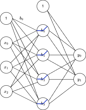
For example, we can express the hidden layer of this network as a matrix multiplication.

\[ \begin{bmatrix} w_{00} & w_{01} & w_{02} \\ w_{10} & w_{11} & w_{12} \\ w_{20} & w_{21} & w_{22} \\ w_{30} & w_{31} & w_{32} \\ \end{bmatrix} \begin{bmatrix} x_{0} \\ x_{1} \\ x_{2} \\ \end{bmatrix} + \begin{bmatrix} b_{0} \\ b_{1} \\ b_{2} \\ b_{3} \\ \end{bmatrix} = \begin{bmatrix} h_{0} \\ h_{1} \\ h_{2} \\ h_{3} \\ \end{bmatrix} \]

Which we can compute directly on tensors.

import torch

torch.manual_seed(42)

# Define the input tensor (batch size of 1 for simplicity)
input_tensor = torch.tensor([[1.0, 2.0, 3.0]])

# Initialize weights and biases for the hidden layer
weights_hidden = torch.randn(3, 4)  # 3 inputs to 4 hidden nodes
bias_hidden = torch.randn(4)        # 4 hidden nodes

# Initialize weights and biases for the output layer
weights_output = torch.randn(4, 2)  # 4 hidden nodes to 2 outputs
bias_output = torch.randn(2)        # 2 outputs

# Perform matrix multiplication and add biases for the hidden layer
hidden_layer = torch.matmul(input_tensor, weights_hidden) + bias_hidden

# Apply ReLU activation function
hidden_layer_activated = torch.relu(hidden_layer)

# Perform matrix multiplication and add biases for the output layer
output_layer = torch.matmul(hidden_layer_activated, weights_output) + bias_output

print("Output:", output_layer)

Output: tensor([[7.4129, 6.0104]])

Let’s look at the matrix equations.

Here’s the calculation of the hidden layer.

Code

latex_input_tensor = tensor_to_latex(input_tensor.T)
latex_weights_hidden = tensor_to_latex(weights_hidden.T)
latex_bias_hidden = tensor_to_latex(bias_hidden)
latex_weights_output = tensor_to_latex(weights_output.T)
latex_bias_output = tensor_to_latex(bias_output)
latex_hidden_layer = tensor_to_latex(hidden_layer.T)
latex_hidden_layer_activated = tensor_to_latex(hidden_layer_activated.T)
latex_output_layer = tensor_to_latex(output_layer.T)

# display(Math(f"\\text{{input tensor}} = {latex_input_tensor}"))
# display(Math(f"\\text{{weights hidden}} = {latex_weights_hidden}"))
# display(Math(f"\\text{{bias hidden}} = {latex_bias_hidden}"))
# display(Math(f"\\text{{weights output}} = {latex_weights_output}"))
# display(Math(f"\\text{{bias output}} = {latex_bias_output}"))
# display(Math(f"\\text{{hidden layer}} = {latex_hidden_layer}"))
# display(Math(f"\\text{{hidden layer activated}} = {latex_hidden_layer_activated}"))
# display(Math(f"\\text{{output layer}} = {latex_output_layer}"))

display(Math(f"{latex_weights_hidden} \\times {latex_input_tensor} + {latex_bias_hidden} = {latex_hidden_layer}"))

\(\displaystyle \begin{bmatrix} 0.34 & -1.12 & 0.46 \\ 0.13 & -0.19 & 0.27 \\ 0.23 & 2.21 & 0.53 \\ 0.23 & -0.64 & 0.81 \\ \end{bmatrix} \times \begin{bmatrix} 1.00 \\ 2.00 \\ 3.00 \\ \end{bmatrix} + \begin{bmatrix} 1.11 \\ -1.69 \\ -0.99 \\ 0.96 \\ \end{bmatrix} = \begin{bmatrix} 0.59 \\ -1.13 \\ 5.27 \\ 2.34 \\ \end{bmatrix}\)

Then we apply the ReLU activation function.

Code

display(Math(f"\\mathrm{{ReLU}}({latex_hidden_layer}) = {latex_hidden_layer_activated}"))

\(\displaystyle \mathrm{ReLU}(\begin{bmatrix} 0.59 \\ -1.13 \\ 5.27 \\ 2.34 \\ \end{bmatrix}) = \begin{bmatrix} 0.59 \\ 0.00 \\ 5.27 \\ 2.34 \\ \end{bmatrix}\)

And finally we calculate the output linear layer.

Code

display(Math(f"{latex_weights_output} \\times {latex_hidden_layer_activated} + {latex_bias_output} = {latex_output_layer}"))

\(\displaystyle \begin{bmatrix} 1.32 & -0.77 & 1.35 & -0.33 \\ 0.82 & -0.75 & 0.69 & 0.79 \\ \end{bmatrix} \times \begin{bmatrix} 0.59 \\ 0.00 \\ 5.27 \\ 2.34 \\ \end{bmatrix} + \begin{bmatrix} 0.28 \\ 0.06 \\ \end{bmatrix} = \begin{bmatrix} 7.41 \\ 6.01 \\ \end{bmatrix}\)

Fully Connected Layer with Batched Input

With no change to the previous code, we can now process a batch of inputs.

import torch

torch.manual_seed(42)

# Define the input tensor (batch size of 5)
input_tensor = torch.tensor([[1.0, 2.0, 3.0], [4.0, 5.0, 6.0], [7.0, 8.0, 9.0], [10.0, 11.0, 12.0], [13.0, 14.0, 15.0]])

#vvvv The code below is the same as above ^^^^^

# Initialize weights and biases for the hidden layer
weights_hidden = torch.randn(3, 4)  # 3 inputs to 4 hidden nodes
bias_hidden = torch.randn(4)        # 4 hidden nodes

# Initialize weights and biases for the output layer
weights_output = torch.randn(4, 2)  # 4 hidden nodes to 2 outputs
bias_output = torch.randn(2)        # 2 outputs

# Perform matrix multiplication and add biases for the hidden layer
hidden_layer = torch.matmul(input_tensor, weights_hidden) + bias_hidden

# Apply ReLU activation function
hidden_layer_activated = torch.relu(hidden_layer)

# Perform matrix multiplication and add biases for the output layer
output_layer = torch.matmul(hidden_layer_activated, weights_output) + bias_output

print("Output:", output_layer)

Output: tensor([[ 7.4129,  6.0104],
        [18.3247, 12.6200],
        [29.9141, 19.6131],
        [41.1189, 26.2293],
        [52.3238, 32.8455]])

PyTorch 01 - Tensors

PyTorch Introduction

Key Features of PyTorch

PyTorch vs TensorFlow

Key Differences

PyTorch

TensorFlow

Tutorial

Tensors

Tensor Creation

Operations on Tensors

Standard numpy-like indexing and slicing

Joining tensors

Matrix Multiplication

Equivalent matrix multiplication operations

Method 1: Use the `@` matrix multiplication operator

Method 2: call `.matmul` method on the tensor

Method 3: Call the `torch.matmul` function with the two input operands and the output tensor.

Vector Dot Product

Matrix-Vector Multiplication

Batched Matrix Multiplication

Batched Matrix x Broadcasted Vector

Batched Matrix x Batched Matrix

Batched Matrix x Broadcasted Matrix

Element-wise Multiplication

Fully Connected Layer as Matrix Multiplication

Fully Connected Layer with Batched Input

Further Reading

References

PyTorch Introduction

Key Features of PyTorch

PyTorch vs TensorFlow

Key Differences

PyTorch

TensorFlow

Tutorial

Tensors

Tensor Creation

Operations on Tensors

Standard numpy-like indexing and slicing

Joining tensors

Matrix Multiplication

Equivalent matrix multiplication operations

Method 1: Use the @ matrix multiplication operator

Method 2: call .matmul method on the tensor

Method 3: Call the torch.matmul function with the two input operands and the output tensor.

Vector Dot Product

Matrix-Vector Multiplication

Batched Matrix Multiplication

Batched Matrix x Broadcasted Vector

Batched Matrix x Batched Matrix

Batched Matrix x Broadcasted Matrix

Element-wise Multiplication

Fully Connected Layer as Matrix Multiplication

Fully Connected Layer with Batched Input

Further Reading

References

Method 1: Use the `@` matrix multiplication operator

Method 2: call `.matmul` method on the tensor

Method 3: Call the `torch.matmul` function with the two input operands and the output tensor.