import torch
from torch import nn
from torch.utils.data import DataLoader
from torchvision import datasets
from torchvision.transforms import ToTensor

training_data = datasets.CIFAR10(
    root="data",
    train=True,
    download=True,
    transform=ToTensor()
)

test_data = datasets.CIFAR10(
    root="data",
    train=False,
    download=True,
    transform=ToTensor()
)

train_dataloader = DataLoader(training_data, batch_size=64)
test_dataloader = DataLoader(test_data, batch_size=64)Introduction
![]()
Based on PyTorch Optimizing Model Parameters
Optimizing Model Parameters
Now that we have a model and data it’s time to train, validate and test our model by optimizing its parameters on our data.
Training a model is an iterative process – in each iteration:
- the model makes a guess about the output,
- calculates the error in its guess (loss),
- collects the derivatives of the error with respect to its parameters (as we saw in the previous section), and
- optimizes these parameters using gradient descent.
For a more detailed walkthrough of this process, check out this video on backpropagation from 3Blue1Brown.
Load Data and Define Model
We load the code from the previous sections on Datasets & DataLoaders and Model Definition.
We’ll use the CIFAR10 dataset again, which consists of 60000 32x32 color images in 10 classes, with 6000 images per class.
Define the model.
class NeuralNetwork(nn.Module):
    def __init__(self):
        super().__init__()
        self.flatten = nn.Flatten()
        self.linear_relu_stack = nn.Sequential(
            nn.Linear(3*32*32, 512),
            nn.ReLU(),
            nn.Linear(512, 512),
            nn.ReLU(),
            nn.Linear(512, 10),
        )

    def forward(self, x):
        x = self.flatten(x)
        logits = self.linear_relu_stack(x)
        return logits
Instantiate the model.
model = NeuralNetwork()Hyperparameters
Hyperparameters
Hyperparameters are adjustable parameters that let you control the model optimization process.
Different hyperparameter values can impact model training and convergence rates.
Read more about hyperparameter tuning with Raytune here.
We define the following hyperparameters for training:
- Number of Epochs - the number times to iterate over the dataset
- Batch Size - the number of data samples propagated through the network before the parameters are updated
- Learning Rate - how much to update models parameters at each batch/epoch.
- Smaller values yield slow learning speed but may get stuck in local minima,
- while large values may result in unpredictable behavior during training by jumping around the solution space.
We’ll choose the following values:
learning_rate = 1e-3
batch_size = 64
epochs = 5
Optimization Loop
Once we set our hyperparameters, we can then train and optimize our model with an optimization loop.
Each iteration of the optimization loop is called an epoch.
Each epoch consists of two main parts:
- The Train Loop - iterate over the training dataset and try to converge to optimal parameters.
- The Validation/Test Loop - iterate over the test dataset to check if model performance is improving.
Let’s briefly familiarize ourselves with some of the concepts used in the training loop.
Loss Function
When presented with some training data, our untrained network will not give the correct answer.
Loss functions measure the degree of dissimilarity of obtained result to the target value, and it is the loss function that we want to minimize during training.
To calculate the loss we make a prediction using the inputs of our given data sample and compare it against the true data label value.
Common loss functions include
- nn.MSELoss (Mean Square Error) for regression tasks, and
- nn.NLLLoss (Negative Log Likelihood) for classification.
- nn.CrossEntropyLoss combines
nn.LogSoftmaxandnn.NLLLoss.
We pass our model’s output logits to nn.CrossEntropyLoss, which will normalize the logits and compute the prediction error.
# Initialize the loss function
loss_fn = nn.CrossEntropyLoss()
Optimizer
Optimization is the process of adjusting model parameters to reduce model error in each training step.
Optimization algorithms define how this process is performed (in this example we use Stochastic Gradient Descent).
All optimization logic is encapsulated in the optimizer object.
Here, we use the SGD optimizer.
There are many different optimizers available in PyTorch such as ADAM and RMSProp, that work better for different kinds of models and data.
We initialize the optimizer by registering the model’s parameters that need to be trained, and passing in the learning rate hyperparameter.
optimizer = torch.optim.SGD(model.parameters(), lr=learning_rate)Inside the training loop, optimization happens in three steps:
- Call
optimizer.zero_grad()to reset the gradients of model parameters. Gradients by default add up; to prevent double-counting, we explicitly zero them at each iteration. - Backpropagate the prediction loss with a call to
loss.backward(). PyTorch deposits the gradients of the loss w.r.t. each parameter. - Once we have our gradients, we call
optimizer.step()to adjust the parameters by the gradients collected in the backward pass.
Full Implementation
We define:
train_loopthat loops over all the data in batches and performs the optimization code, andtest_loopthat evaluates the model’s performance against our test data.
def train_loop(dataloader, model, loss_fn, optimizer, device):
    size = len(dataloader.dataset)
    # Set the model to training mode - important for batch normalization and
    # dropout layers. Unnecessary in this situation but added for best practices
    model.train()
    for batch, (X, y) in enumerate(dataloader):
        # Compute prediction and loss
        pred = model(X.to(device))
        loss = loss_fn(pred, y.to(device))

        # Backpropagation
        loss.backward()
        optimizer.step()

        # BEWARE: We need to zero out the gradients after each iteration because
        # PyTorch accumulates them by default.
        optimizer.zero_grad()

        if batch % 100 == 0:
            loss, current = loss.item(), batch * batch_size + len(X)
            print(f"loss: {loss:>7f}  [{current:>5d}/{size:>5d}]")

    return loss.cpu().detach().numpy()


def test_loop(dataloader, model, loss_fn, device):
    # Set the model to evaluation mode - important for batch normalization and
    # dropout layers. Unnecessary in this situation but added for best practices
    model.eval()
    size = len(dataloader.dataset)
    num_batches = len(dataloader)
    test_loss, correct = 0, 0

    # Evaluating the model with torch.no_grad() ensures that no gradients are
    # computed during test mode. Also serves to reduce unnecessary gradient
    # computations and memory usage for tensors with requires_grad=True
    with torch.no_grad():
        for X, y in dataloader:
            pred = model(X.to(device))
            test_loss += loss_fn(pred, y.to(device)).item()
            correct += (pred.argmax(1) == y.to(device)).type(torch.float).sum().item()

    test_loss /= num_batches
    correct /= size
    print(f"Test Error: \n Accuracy: {(100*correct):>0.1f}%, Avg loss: {test_loss:>8f} \n")

    return test_loss, correct
Feel free to increase the number of epochs to track the model’s improving performance.
learning_rate = 1e-3
batch_size = 64
epochs = 10
We’ll also check if there’s a GPU available and set the device accordingly.
device = (
    "cuda"
    if torch.cuda.is_available()
    else "mps"
    if torch.backends.mps.is_available()
    else "cpu"
)
print(f"Using {device} device")
Using cpu deviceWe initialize the loss function and optimizer, and pass it to train_loop and test_loop and accumulate train and test losses and test accuracy.
import time

# We'll set the random seed for reproducibility of weight initialization
torch.manual_seed(42)

model = NeuralNetwork().to(device)
loss_fn = nn.CrossEntropyLoss()
optimizer = torch.optim.SGD(model.parameters(), lr=learning_rate)

train_losses = []
test_losses = []
test_accuracies = []

start_time = time.time()

for t in range(epochs):
    print(f"Epoch {t+1}\n-------------------------------")
    train_loss = train_loop(train_dataloader, model, loss_fn, optimizer, device)
    test_loss, test_accuracy = test_loop(test_dataloader, model, loss_fn, device)

    train_losses.append(train_loss)
    test_losses.append(test_loss)
    test_accuracies.append(test_accuracy)

print(f"Done! Time taken: {time.time() - start_time:.2f} seconds")
Epoch 1
-------------------------------
loss: 2.309499 [ 64/50000]
loss: 2.310122 [ 6464/50000]
loss: 2.277137 [12864/50000]
loss: 2.292640 [19264/50000]
loss: 2.277530 [25664/50000]
loss: 2.265735 [32064/50000]
loss: 2.281457 [38464/50000]
loss: 2.274072 [44864/50000]
Test Error:
Accuracy: 12.0%, Avg loss: 2.267871
Epoch 2
-------------------------------
loss: 2.287568 [ 64/50000]
loss: 2.283070 [ 6464/50000]
loss: 2.237826 [12864/50000]
loss: 2.262030 [19264/50000]
loss: 2.241528 [25664/50000]
loss: 2.228436 [32064/50000]
loss: 2.253743 [38464/50000]
loss: 2.233874 [44864/50000]
Test Error:
Accuracy: 19.6%, Avg loss: 2.227713
Epoch 3
-------------------------------
loss: 2.253309 [ 64/50000]
loss: 2.247070 [ 6464/50000]
loss: 2.177868 [12864/50000]
loss: 2.227232 [19264/50000]
loss: 2.191311 [25664/50000]
loss: 2.174961 [32064/50000]
loss: 2.222422 [38464/50000]
loss: 2.173692 [44864/50000]
Test Error:
Accuracy: 22.9%, Avg loss: 2.172615
Epoch 4
-------------------------------
loss: 2.208374 [ 64/50000]
loss: 2.196370 [ 6464/50000]
loss: 2.099298 [12864/50000]
loss: 2.184255 [19264/50000]
loss: 2.130482 [25664/50000]
loss: 2.113062 [32064/50000]
loss: 2.193428 [38464/50000]
loss: 2.105793 [44864/50000]
Test Error:
Accuracy: 24.7%, Avg loss: 2.113887
Epoch 5
-------------------------------
loss: 2.162115 [ 64/50000]
loss: 2.144591 [ 6464/50000]
loss: 2.018662 [12864/50000]
loss: 2.141456 [19264/50000]
loss: 2.077917 [25664/50000]
loss: 2.060375 [32064/50000]
loss: 2.175333 [38464/50000]
loss: 2.051365 [44864/50000]
Test Error:
Accuracy: 26.5%, Avg loss: 2.066019
Epoch 6
-------------------------------
loss: 2.124258 [ 64/50000]
loss: 2.105548 [ 6464/50000]
loss: 1.951478 [12864/50000]
loss: 2.104190 [19264/50000]
loss: 2.042454 [25664/50000]
loss: 2.023262 [32064/50000]
loss: 2.158503 [38464/50000]
loss: 2.012434 [44864/50000]
Test Error:
Accuracy: 28.0%, Avg loss: 2.028872
Epoch 7
-------------------------------
loss: 2.094113 [ 64/50000]
loss: 2.077006 [ 6464/50000]
loss: 1.895864 [12864/50000]
loss: 2.072996 [19264/50000]
loss: 2.018962 [25664/50000]
loss: 1.998076 [32064/50000]
loss: 2.137465 [38464/50000]
loss: 1.982371 [44864/50000]
Test Error:
Accuracy: 28.9%, Avg loss: 1.998516
Epoch 8
-------------------------------
loss: 2.068079 [ 64/50000]
loss: 2.053779 [ 6464/50000]
loss: 1.849978 [12864/50000]
loss: 2.047427 [19264/50000]
loss: 2.001680 [25664/50000]
loss: 1.980872 [32064/50000]
loss: 2.114357 [38464/50000]
loss: 1.956221 [44864/50000]
Test Error:
Accuracy: 29.6%, Avg loss: 1.973246
Epoch 9
-------------------------------
loss: 2.043992 [ 64/50000]
loss: 2.033800 [ 6464/50000]
loss: 1.813169 [12864/50000]
loss: 2.026532 [19264/50000]
loss: 1.987598 [25664/50000]
loss: 1.968321 [32064/50000]
loss: 2.092039 [38464/50000]
loss: 1.932983 [44864/50000]
Test Error:
Accuracy: 30.3%, Avg loss: 1.951910
Epoch 10
-------------------------------
loss: 2.020598 [ 64/50000]
loss: 2.015732 [ 6464/50000]
loss: 1.782849 [12864/50000]
loss: 2.008502 [19264/50000]
loss: 1.975001 [25664/50000]
loss: 1.958090 [32064/50000]
loss: 2.071905 [38464/50000]
loss: 1.911957 [44864/50000]
Test Error:
Accuracy: 31.0%, Avg loss: 1.933615
Done! Time taken: 107.79 secondsFinally, we plot the train and test losses and test accuracy.
import matplotlib.pyplot as plt

# Plotting the results
epochs_range = range(1, epochs + 1)
plt.figure(figsize=(12, 4))

plt.subplot(1, 2, 1)
plt.plot(epochs_range, train_losses, label='Train Loss')
plt.plot(epochs_range, test_losses, label='Test Loss')
plt.xlabel('Epochs')
plt.ylabel('Loss')
plt.title('Train and Test Loss')
plt.legend()

plt.subplot(1, 2, 2)
plt.plot(epochs_range, test_accuracies, label='Test Accuracy')
plt.xlabel('Epochs')
plt.ylabel('Accuracy')
plt.title('Test Accuracy')
plt.legend()

plt.tight_layout()
plt.show()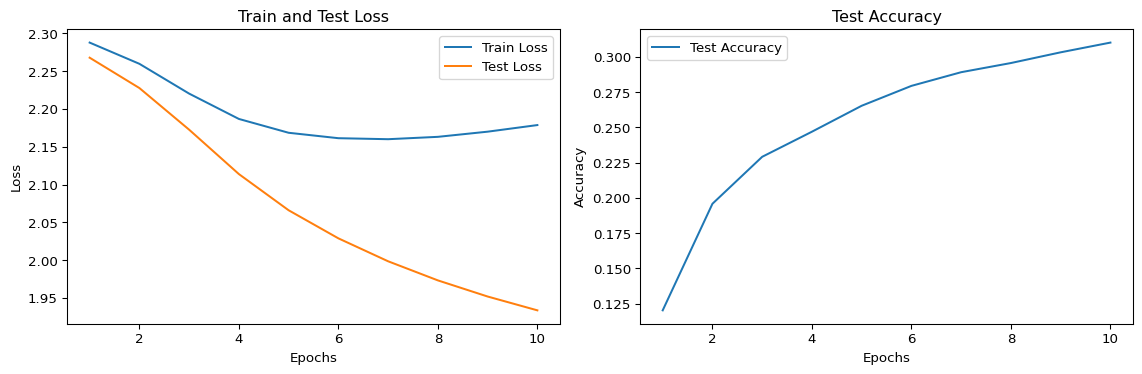
It’s curious that the test loss is lower than the train loss and that the train loss stops decreasing around epoch 6.
Challenge: Play around with the hyperparameters and see if you can get training loss lower than the test loss and continue to decrease.