Code
import os
import torch
from torch import nn
from torch.utils.data import DataLoader
from torchvision import datasets, transforms![]()
Based on PyTorch Build Model Tutorial.
Neural networks comprise of layers/modules that perform operations on data.
The torch.nn namespace provides all the building blocks you need to build your own neural network.
Every module in PyTorch subclasses the nn.Module.
A neural network is a module itself that consists of other modules (layers). This nested structure allows for building and managing complex architectures easily.
In the following sections, we’ll build a neural network to classify images like those in the CIFAR-10 dataset.
import os
import torch
from torch import nn
from torch.utils.data import DataLoader
from torchvision import datasets, transformsWe want to be able to train our model on a hardware accelerator like the GPU or MPS, if available.
Let’s check to see if
are available, otherwise we use the CPU.
device = (
    "cuda"
    if torch.cuda.is_available()
    else "mps"
    if torch.backends.mps.is_available()
    else "cpu"
)
print(f"Using {device} device")
Using cpu deviceWe define our neural network by subclassing nn.Module, and initialize the neural network layers in __init__.
Every nn.Module subclass implements the operations on input data in the forward method.
class NeuralNetwork(nn.Module):
    def __init__(self):
        super().__init__()
        self.flatten = nn.Flatten()
        self.linear_relu_stack = nn.Sequential(
            nn.Linear(3*32*32, 512),
            nn.ReLU(),
            nn.Linear(512, 512),
            nn.ReLU(),
            nn.Linear(512, 10),
        )

    def forward(self, x):
        x = self.flatten(x)
        logits = self.linear_relu_stack(x)
        return logits
We create an instance of NeuralNetwork, and move it to the device, and print its structure.
model = NeuralNetwork().to(device)
print(model)
NeuralNetwork(
(flatten): Flatten(start_dim=1, end_dim=-1)
(linear_relu_stack): Sequential(
(0): Linear(in_features=3072, out_features=512, bias=True)
(1): ReLU()
(2): Linear(in_features=512, out_features=512, bias=True)
(3): ReLU()
(4): Linear(in_features=512, out_features=10, bias=True)
)
)Note that this is an untrained model with randomly initialized weights.
Keras has a nicer way to print the model architecture. To do something similar in PyTorch, you can use torchinfo package.
from torchinfo import summary
summary(model, input_size=(1, 3, 32, 32))
==========================================================================================
Layer (type:depth-idx) Output Shape Param #
==========================================================================================
NeuralNetwork [1, 10] --
├─Flatten: 1-1 [1, 3072] --
├─Sequential: 1-2 [1, 10] --
│ └─Linear: 2-1 [1, 512] 1,573,376
│ └─ReLU: 2-2 [1, 512] --
│ └─Linear: 2-3 [1, 512] 262,656
│ └─ReLU: 2-4 [1, 512] --
│ └─Linear: 2-5 [1, 10] 5,130
==========================================================================================
Total params: 1,841,162
Trainable params: 1,841,162
Non-trainable params: 0
Total mult-adds (Units.MEGABYTES): 1.84
==========================================================================================
Input size (MB): 0.01
Forward/backward pass size (MB): 0.01
Params size (MB): 7.36
Estimated Total Size (MB): 7.39
==========================================================================================# the torchinfo package seems to move the model to the CPU so reinitializing
model = NeuralNetwork().to(device)To use the model, we pass it the input data.
This executes the model’s forward.
Do not call model.forward() directly!
X = torch.rand(1, 3, 32, 32, device=device)
logits = model(X)
# print(f"Logits: {logits.T}")
print(f"Logits size: {logits.size()}")
Logits size: torch.Size([1, 10])Calling the model on the input returns a \(1\times10\) tensor corresponding to each output of 10 raw predicted values for each class
Note that we had to set the batch size to 1 on the input, e.g. a \(1\times3\times32\times32\) tensor.
That’s because nn.Flatten is batch aware, i.e. it flattens each image in the batch individually.
We get the prediction probabilities by passing it through an instance of the nn.Softmax module.
pred_probab = nn.Softmax(dim=1)(logits)
# print(f"\nPredicted probabilities: {pred_probab.T}")
And then we get the predicted class by choosing the index with the maximum probability.
y_pred = pred_probab.argmax(1)
print(f"Predicted class: {y_pred}")
Predicted class: tensor([3])\(\displaystyle \mathrm{logits} = \begin{bmatrix} -0.009 \\ 0.040 \\ -0.033 \\ 0.124 \\ -0.028 \\ 0.067 \\ -0.047 \\ -0.091 \\ 0.031 \\ 0.012 \\ \end{bmatrix}, \quad \mathrm{pred\_probab} = \begin{bmatrix} 0.098 \\ 0.103 \\ 0.096 \\ 0.112 \\ 0.096 \\ 0.106 \\ 0.095 \\ 0.091 \\ 0.102 \\ 0.100 \\ \end{bmatrix}\)
Let’s step through the layers in the model one by one.
To illustrate it, we will create a sample minibatch of 5 “images” with random values of size 32x32 and see what happens to it as we pass it through the network.
input_image = torch.rand(5,3,32,32)
print(input_image.size())
torch.Size([5, 3, 32, 32])We initialize the nn.Flatten layer to convert each 2D 3x32x32 image into a contiguous array of 3072 pixel values (the minibatch dimension (at dim=0) is maintained).
flatten = nn.Flatten()
flat_image = flatten(input_image)
print(flat_image.size())
torch.Size([5, 3072])The linear layer is a module that applies a linear transformation on the input using its stored weights and biases.
Remember from our Tensor discussions that the linear calculation for the linear fully connected layer as in the following figure
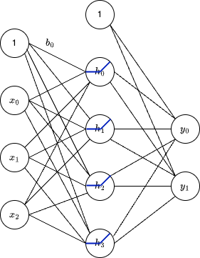
can be expressed as a matrix multiplication.
\[ \begin{bmatrix} w_{00} & w_{01} & w_{02} \\ w_{10} & w_{11} & w_{12} \\ w_{20} & w_{21} & w_{22} \\ w_{30} & w_{31} & w_{32} \\ \end{bmatrix} \begin{bmatrix} x_{0} \\ x_{1} \\ x_{2} \\ \end{bmatrix} + \begin{bmatrix} b_{0} \\ b_{1} \\ b_{2} \\ b_{3} \\ \end{bmatrix} = \begin{bmatrix} h_{0} \\ h_{1} \\ h_{2} \\ h_{3} \\ \end{bmatrix} \]
In the example below the weights matrix is \(20\times3072\) and the bias vector is \(20\times1\).
layer1 = nn.Linear(in_features=3*32*32, out_features=20)
hidden1 = layer1(flat_image)
print(hidden1.size())
torch.Size([5, 20])We get a 5 batches of 20 values each in a \(5\times20\) tensor.
Non-linear activations are what create the complex mappings between the model’s inputs and outputs.
They are applied after linear transformations to introduce nonlinearity, helping neural networks learn a wide variety of phenomena.
Without non-linear activations, the model would just be a linear function.
Later we’ll see that adding non-linearities make neural networks “Universal Approximators”.
In this model, we use nn.ReLU between our linear layers, but there are other activations to introduce non-linearity in your model.
The ReLU activation function is defined as \(ReLU(x) = \max(0, x)\).
import matplotlib.pyplot as plt
import numpy as np

# Generate values between -5 and 5
x = np.linspace(-5, 5, 100)

# Apply ReLU function
tensor_x = torch.tensor(x)
tensor_y = nn.ReLU()(tensor_x)
y = tensor_y.numpy()

# or equivalently
# y = nn.ReLU()(torch.tensor(x)).numpy()

# Plot the ReLU function
plt.figure(figsize=(8, 6))
plt.plot(x, y, label="ReLU(x)")
plt.title("ReLU Activation Function")
plt.xlabel("Input")
plt.ylabel("Output")
plt.legend()
plt.grid(True)
plt.show()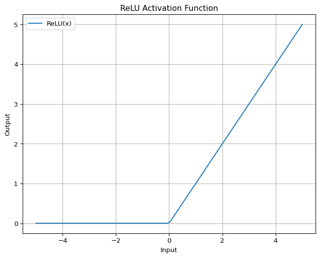
print(f"Before ReLU: {hidden1}\n\n")
hidden1 = nn.ReLU()(hidden1)
print(f"After ReLU: {hidden1}")
Before ReLU: tensor([[ 3.5366e-01, 2.1987e-01, 4.2610e-02, -3.6928e-01, 1.3681e-01,
5.0700e-02, -1.8924e-01, 4.2756e-01, 3.7748e-04, -3.4086e-01,
-9.8638e-02, -4.4003e-02, 1.9676e-02, -6.3249e-02, 2.9013e-01,
-6.2108e-02, -2.2507e-01, 3.6948e-01, -3.1360e-01, -1.7534e-01],
[ 3.5173e-01, 1.7327e-02, -3.9511e-01, -1.9200e-01, -4.5213e-02,
3.3204e-02, 6.7871e-04, 3.5538e-01, 3.8391e-01, -4.9995e-01,
-5.3946e-02, -3.0964e-01, -1.6902e-01, 1.5205e-01, 3.2393e-01,
-3.3394e-01, 2.2958e-02, 6.9104e-02, 9.1648e-02, 1.5339e-02],
[ 5.0777e-01, -5.5668e-02, -5.4693e-01, -7.9588e-02, -4.2518e-01,
-1.4591e-01, 1.7362e-01, 5.1331e-01, 2.3288e-01, -3.1589e-02,
4.8346e-01, -2.0554e-01, -3.6604e-02, 9.3143e-02, 3.4133e-01,
-3.9281e-01, -1.4013e-01, 1.7305e-02, 1.1533e-01, 2.6788e-01],
[ 3.7084e-01, 1.7047e-01, -2.5854e-01, -7.9995e-02, 1.6883e-02,
7.8726e-02, 5.6937e-02, 3.3519e-01, 1.5630e-01, -4.4544e-01,
-8.1628e-02, -5.3962e-02, 1.2000e-01, 9.6353e-02, 3.4097e-01,
-1.7409e-01, -2.5916e-02, 3.5993e-01, -1.2485e-01, 8.0006e-02],
[ 1.1626e-01, -3.7589e-01, -6.1218e-02, -1.7161e-01, 2.9600e-02,
1.4925e-01, 2.6728e-01, 3.7037e-01, 2.6949e-01, -6.7148e-01,
-1.5290e-01, -9.2789e-02, 2.7987e-02, 2.2977e-01, 5.0134e-01,
-1.7159e-01, 5.9841e-02, 1.0535e-01, -2.1276e-01, 4.6140e-02]],
grad_fn=<AddmmBackward0>)
After ReLU: tensor([[3.5366e-01, 2.1987e-01, 4.2610e-02, 0.0000e+00, 1.3681e-01, 5.0700e-02,
0.0000e+00, 4.2756e-01, 3.7748e-04, 0.0000e+00, 0.0000e+00, 0.0000e+00,
1.9676e-02, 0.0000e+00, 2.9013e-01, 0.0000e+00, 0.0000e+00, 3.6948e-01,
0.0000e+00, 0.0000e+00],
[3.5173e-01, 1.7327e-02, 0.0000e+00, 0.0000e+00, 0.0000e+00, 3.3204e-02,
6.7871e-04, 3.5538e-01, 3.8391e-01, 0.0000e+00, 0.0000e+00, 0.0000e+00,
0.0000e+00, 1.5205e-01, 3.2393e-01, 0.0000e+00, 2.2958e-02, 6.9104e-02,
9.1648e-02, 1.5339e-02],
[5.0777e-01, 0.0000e+00, 0.0000e+00, 0.0000e+00, 0.0000e+00, 0.0000e+00,
1.7362e-01, 5.1331e-01, 2.3288e-01, 0.0000e+00, 4.8346e-01, 0.0000e+00,
0.0000e+00, 9.3143e-02, 3.4133e-01, 0.0000e+00, 0.0000e+00, 1.7305e-02,
1.1533e-01, 2.6788e-01],
[3.7084e-01, 1.7047e-01, 0.0000e+00, 0.0000e+00, 1.6883e-02, 7.8726e-02,
5.6937e-02, 3.3519e-01, 1.5630e-01, 0.0000e+00, 0.0000e+00, 0.0000e+00,
1.2000e-01, 9.6353e-02, 3.4097e-01, 0.0000e+00, 0.0000e+00, 3.5993e-01,
0.0000e+00, 8.0006e-02],
[1.1626e-01, 0.0000e+00, 0.0000e+00, 0.0000e+00, 2.9600e-02, 1.4925e-01,
2.6728e-01, 3.7037e-01, 2.6949e-01, 0.0000e+00, 0.0000e+00, 0.0000e+00,
2.7987e-02, 2.2977e-01, 5.0134e-01, 0.0000e+00, 5.9841e-02, 1.0535e-01,
0.0000e+00, 4.6140e-02]], grad_fn=<ReluBackward0>)Although not technically a layer, nn.Sequential is an ordered container of modules and can be treated as a layer.
The data is passed through all the modules in the same order as defined. You can use sequential containers to put together a quick network like seq_modules.
seq_modules = nn.Sequential(
    flatten,
    layer1,
    nn.ReLU(),
    nn.Linear(20, 10)
)
input_image = torch.rand(5,3,32,32)
logits = seq_modules(input_image)The last linear layer of the neural network returns logits - raw values in \((-\infty, \infty)\) - which are passed to the nn.Softmax module.
The softmax function is defined as
\[ \mathrm{Softmax}(x_{i}) = \frac{e^{x_i}}{\sum_j e^{x_j}} \]
The logits are scaled to values \([0, 1]\) representing the model’s predicted probabilities for each class. dim parameter indicates the dimension along which the values must sum to 1.
softmax = nn.Softmax(dim=1)
pred_probab = softmax(logits)
print(f"Softmax size: {pred_probab.size()}")
Softmax size: torch.Size([5, 10])Many layers inside a neural network are parameterized, i.e. have associated weights and biases that are optimized during training.
Subclassing nn.Module automatically tracks all fields defined inside your model object, and makes all parameters accessible using your model’s parameters() or named_parameters() methods.
In this example, we iterate over each parameter, and print its size and a preview of its values.
print(f"Model structure: {model}\n\n")

for name, param in model.named_parameters():
    print(f"Layer: {name} | Size: {param.size()}") # | Values : {param[:2]} \n")
Model structure: NeuralNetwork(
(flatten): Flatten(start_dim=1, end_dim=-1)
(linear_relu_stack): Sequential(
(0): Linear(in_features=3072, out_features=512, bias=True)
(1): ReLU()
(2): Linear(in_features=512, out_features=512, bias=True)
(3): ReLU()
(4): Linear(in_features=512, out_features=10, bias=True)
)
)
Layer: linear_relu_stack.0.weight | Size: torch.Size([512, 3072])
Layer: linear_relu_stack.0.bias | Size: torch.Size([512])
Layer: linear_relu_stack.2.weight | Size: torch.Size([512, 512])
Layer: linear_relu_stack.2.bias | Size: torch.Size([512])
Layer: linear_relu_stack.4.weight | Size: torch.Size([10, 512])
Layer: linear_relu_stack.4.bias | Size: torch.Size([10])We can count the sizes of the matrices and vectors to verify that the number of parameters in the model agrees with the summary printed earlier.
print(f"{512*3072 + 512 + 512*512 + 512 + 512*10 + 10:,}")1,841,162Let’s load the CIFAR-10 training data so we can apply our model to it.
import torch
from torch.utils.data import Dataset
from torchvision import datasets
from torchvision.transforms import ToTensor
import matplotlib.pyplot as plt

training_data = datasets.CIFAR10(
    root="data",
    train=True,
    download=True,
    transform=ToTensor()
)
We can then select a random sample from the training data and print its shape, type, and label.
sample_idx = torch.randint(len(training_data), size=(1,)).item()
img, label = training_data[sample_idx]

print(f"Sample index: {sample_idx}")
print(f"Label: {label}")
print(f"img.shape: {img.shape}")
print(f"img.dtype: {img.dtype}")
Sample index: 691
Label: 3
img.shape: torch.Size([3, 32, 32])
img.dtype: torch.float32We can then create a DataLoader to load the data in batches.
from torch.utils.data import DataLoader
train_dataloader = DataLoader(training_data, batch_size=5, shuffle=True)
Let’s grab one batch of images and labels and print their shapes.
# Display image and label.
train_features, train_labels = next(iter(train_dataloader))
print(f"Feature batch shape: {train_features.size()}")
print(f"Labels batch shape: {train_labels.size()}")
Feature batch shape: torch.Size([5, 3, 32, 32])
Labels batch shape: torch.Size([5])labels_map = {
0: "plane",
1: "car",
2: "bird",
3: "cat",
4: "deer",
5: "dog",
6: "frog",
7: "horse",
8: "ship",
9: "truck",
}
import matplotlib.pyplot as plt
fig, axes = plt.subplots(1, 5, figsize=(15, 3))
for i in range(5):
img = train_features[i].squeeze() # squeeze() removes dimension of size 1, e.g. (1, 3, 32, 32) -> (3, 32, 32)
label = train_labels[i]
axes[i].imshow(img.permute(1, 2, 0))
axes[i].set_title(labels_map[label.item()])
axes[i].axis('off')
plt.show()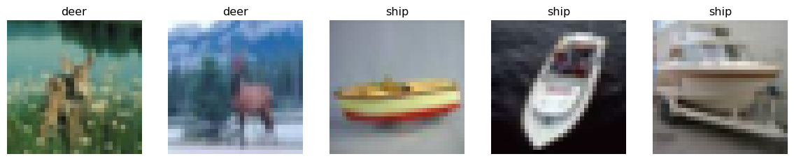
Let’s instantiate our model again and move it to the device.
model = NeuralNetwork().to(device)We can then pass the batch of images through the model and print the size of the logits.
Note that we had to move the tensor representing thebatch of images to the device.
logits = model(train_features.to(device))
print(f"Logits size: {logits.size()}")
Logits size: torch.Size([5, 10])And finally, we can pass the logits through the softmax function to get the predicted probabilities.
softmax = nn.Softmax(dim=1)
pred_probab = softmax(logits)
print(f"Softmax size: {pred_probab.size()}")
Softmax size: torch.Size([5, 10])\(\displaystyle \mathrm{logits} = \begin{bmatrix} 0.011 & -0.017 & 0.005 & 0.014 & -0.024 \\ 0.048 & 0.044 & 0.083 & 0.082 & 0.068 \\ -0.015 & 0.046 & 0.022 & 0.006 & -0.020 \\ -0.049 & -0.061 & -0.057 & -0.062 & -0.037 \\ -0.090 & -0.051 & -0.046 & -0.112 & -0.056 \\ -0.009 & -0.022 & -0.027 & -0.029 & -0.031 \\ 0.049 & 0.033 & 0.028 & 0.032 & 0.033 \\ 0.079 & 0.067 & 0.095 & 0.055 & 0.079 \\ 0.059 & 0.076 & 0.085 & 0.102 & 0.056 \\ 0.066 & 0.068 & 0.034 & 0.052 & 0.082 \\ \end{bmatrix}, \quad \mathrm{pred\_probab} = \begin{bmatrix} 0.099 & 0.096 & 0.098 & 0.100 & 0.096 \\ 0.103 & 0.102 & 0.106 & 0.107 & 0.105 \\ 0.097 & 0.103 & 0.100 & 0.099 & 0.096 \\ 0.094 & 0.092 & 0.092 & 0.092 & 0.095 \\ 0.090 & 0.093 & 0.093 & 0.088 & 0.093 \\ 0.098 & 0.096 & 0.095 & 0.096 & 0.095 \\ 0.103 & 0.101 & 0.100 & 0.102 & 0.102 \\ 0.106 & 0.105 & 0.107 & 0.104 & 0.106 \\ 0.104 & 0.106 & 0.106 & 0.109 & 0.104 \\ 0.105 & 0.105 & 0.101 & 0.104 & 0.107 \\ \end{bmatrix}\)
And like before we get the predicted class by choosing the index with the maximum probability.
y_pred = pred_probab.argmax(1)
print(f"Predicted class: {y_pred}")
Predicted class: tensor([7, 8, 7, 8, 9])And of course we are not getting the right predictions yet because we have not trained the model!
Of course, in practice we would use other types of layers, e.g. convolutions, dropout, batch normalization, etc., especially for image data.